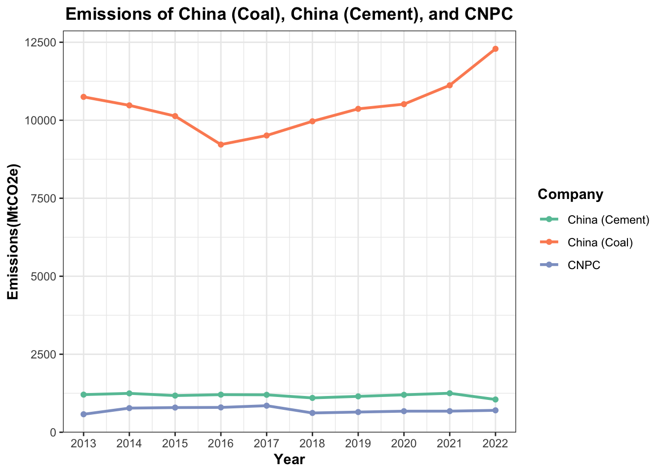
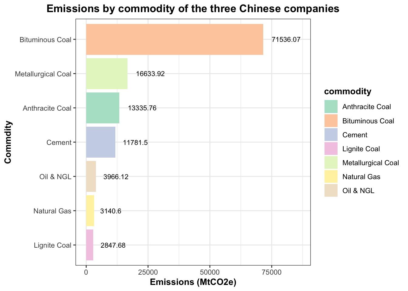
Q5: For the recent 10 years, for the emissions of China (Coal), China (Cement) and CNPC, which commodity has contributed most emissions?
df_cleaned|>filter(year>="2013" )|>filter(company %in%c("China (Coal)", "China (Cement)","CNPC"))|>group_by(commodity)|>summarise(n=sum(emissions))|>ggplot(aes(x =fct_reorder(commodity,n), y = n,fill = commodity)) +geom_col() +geom_col(width =0.7) +coord_flip() +scale_fill_brewer(palette ="Pastel2") +labs(title ="Emissions by commodity of the three Chinese companies",x ="Commdity",y ="Emissions (MtCO2e)")+theme_bw()+# Add values to the chart.geom_text(aes(label = n),hjust =-0.3, size =3)+theme(plot.title =element_text(hjust =0.5, face ="bold"),legend.position ="right",legend.title =element_text(face ="bold"),axis.title =element_text(face ="bold"))+# Extends the range of the y-axis so that it is larger than the actual data range, leaving more space for the labels.expand_limits(y =c(0, max(df_cleaned$emissions) *10))
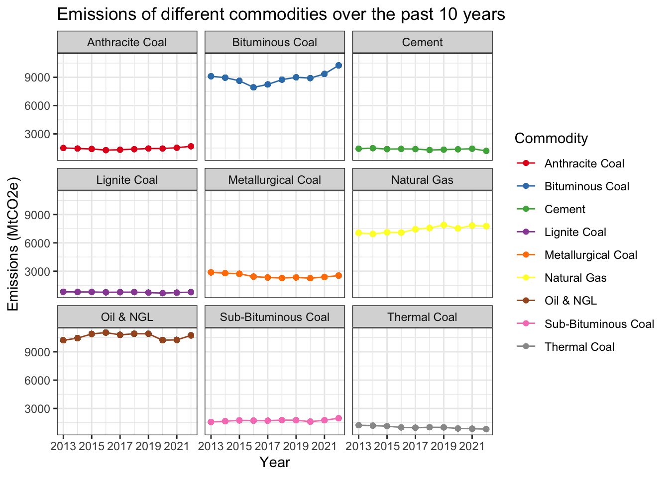
df_cleaned|>filter(year>="2013" )|>group_by(year,commodity)|>mutate(each_emissions=sum(emissions))|>ggplot(aes(x = year, y = each_emissions, color = commodity)) +geom_line(aes(color = commodity)) +geom_point(aes(color = commodity)) +scale_x_continuous(breaks =seq(2013, 2022, by =2)) +scale_color_brewer(palette ="Set1") +labs(title ="Emissions of different commodities over the past 10 years",x ="Year",y ="Emissions (MtCO2e)",color ="Commodity") +facet_wrap(~commodity) +theme_bw()
Q8
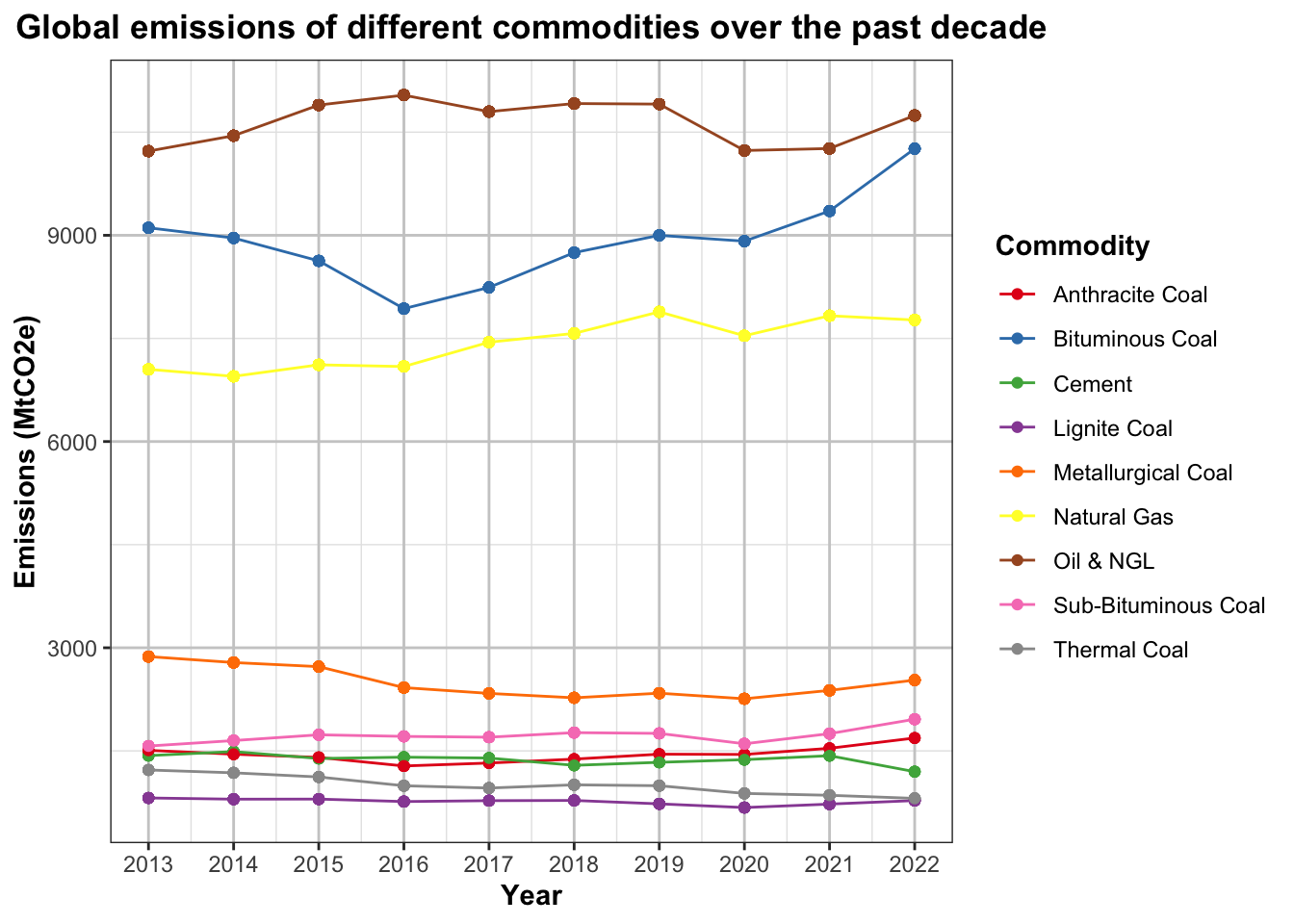
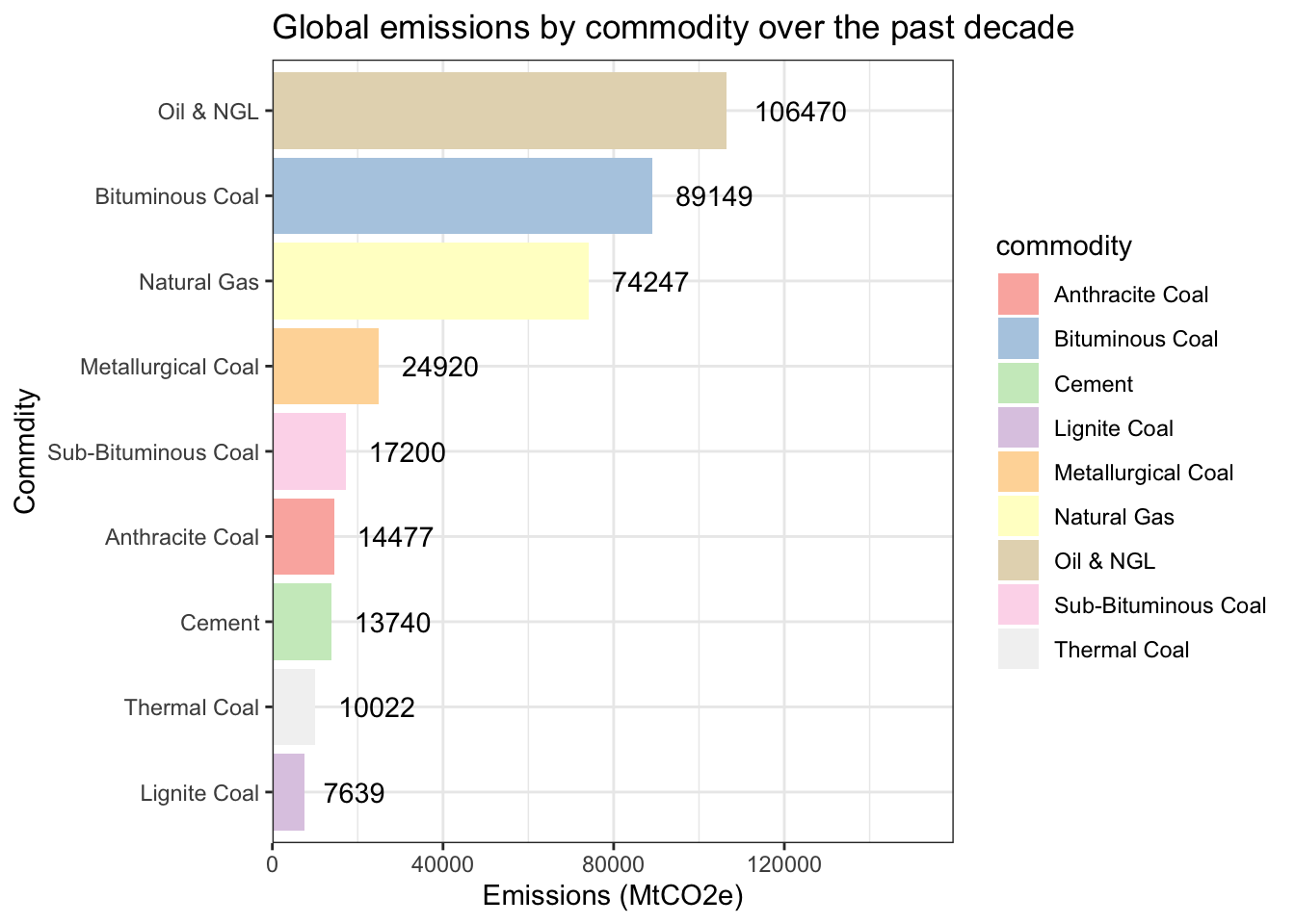
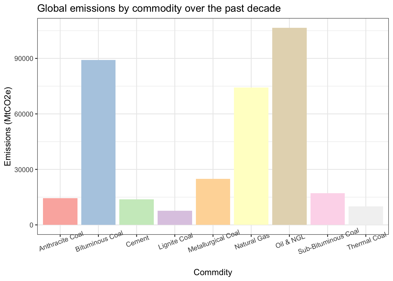
Q8: For the recent 10 years, what are the total emissions for each type of commodity?
df_cleaned|>filter(year>="2013" )|>group_by(commodity)|>summarise(each_emissions=sum(emissions))|>ggplot(aes(x =fct_reorder(commodity,each_emissions), y = each_emissions,fill = commodity)) +geom_col() +geom_col(width =0.7) +# Use the geom_text function to add values to the bar chart.geom_text(aes(label =round(each_emissions)), hjust =-0.3, size =3.8) +coord_flip() +scale_fill_brewer(palette ="Pastel1") +labs(title ="Global emissions by commodity over the past decade",x ="Commdity",y ="Emissions (MtCO2e)")+theme_bw()+# Extends the range of the y-axis so that it is larger than the actual data range, leaving more space for the labels.scale_y_continuous(expand =expansion(mult =c(0,0.5)))
df_cleaned|>filter(year>="2013" )|>group_by(commodity)|>summarise(each_emissions=sum(emissions))|>ggplot(aes(x = commodity, y = each_emissions,fill = commodity)) +geom_col() +geom_col(width =0.5) +scale_fill_brewer(palette ="Pastel1") +labs(title ="Global emissions by commodity over the past decade",x ="Commdity",y ="Emissions (MtCO2e)")+theme_bw()+# Remove the unnecessary legend and adjust the angle of the commodities to avoid words overlap.theme(legend.position ="none",axis.text.x =element_text(angle =20),hjust=2)
Warning in plot_theme(plot): The `hjust` theme element is not defined in the
element hierarchy.
Q9
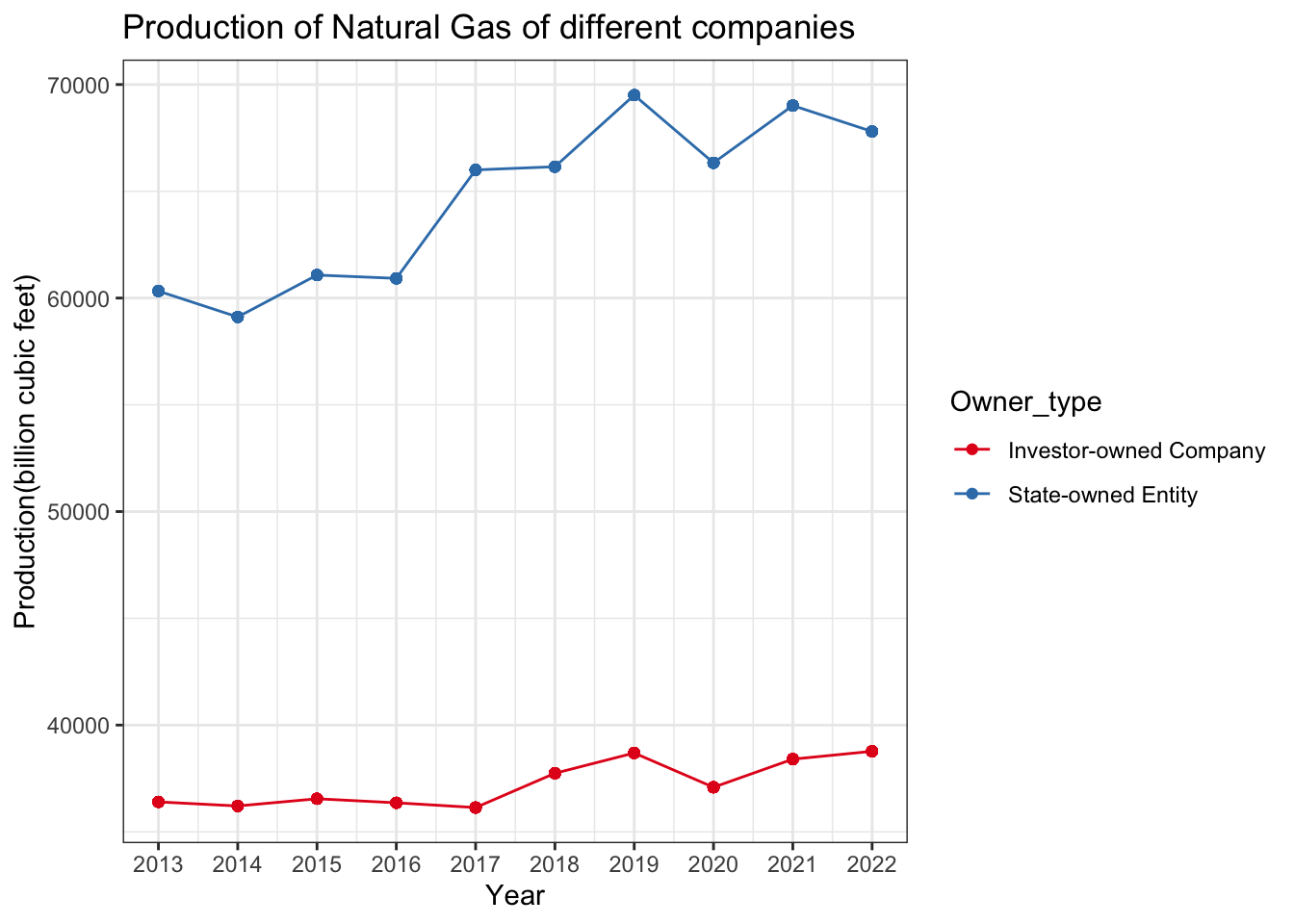
Q9: For Natural Gas, over the past decade, calculate the quantity produced by companies of different owner_type in each year.
df_cleaned|>filter(year>="2013",commodity=="Natural Gas" )|>group_by(year,owner_type)|>mutate(total_production=sum(quantity))|>ggplot(aes(x = year, y = total_production, color = owner_type)) +geom_line(aes(color = owner_type)) +geom_point(aes(color = owner_type)) +scale_x_continuous(breaks =seq(2013, 2022, 1)) +scale_color_brewer(palette ="Set1") +labs(title ="Production of Natural Gas of different companies",x ="Year",y ="Production(billion cubic feet)",color ="Owner_type") +theme_bw()
Q10
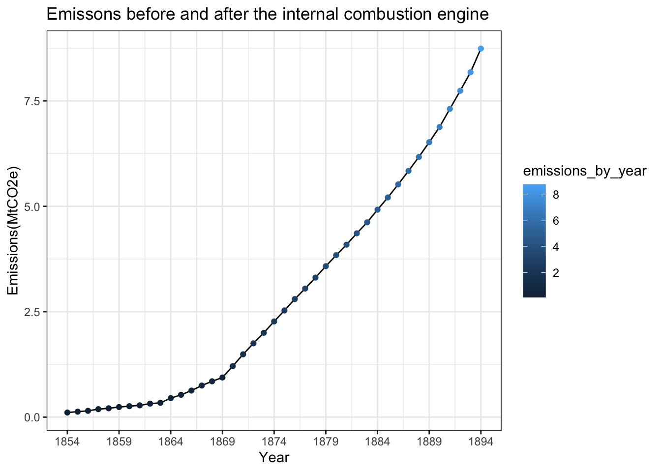
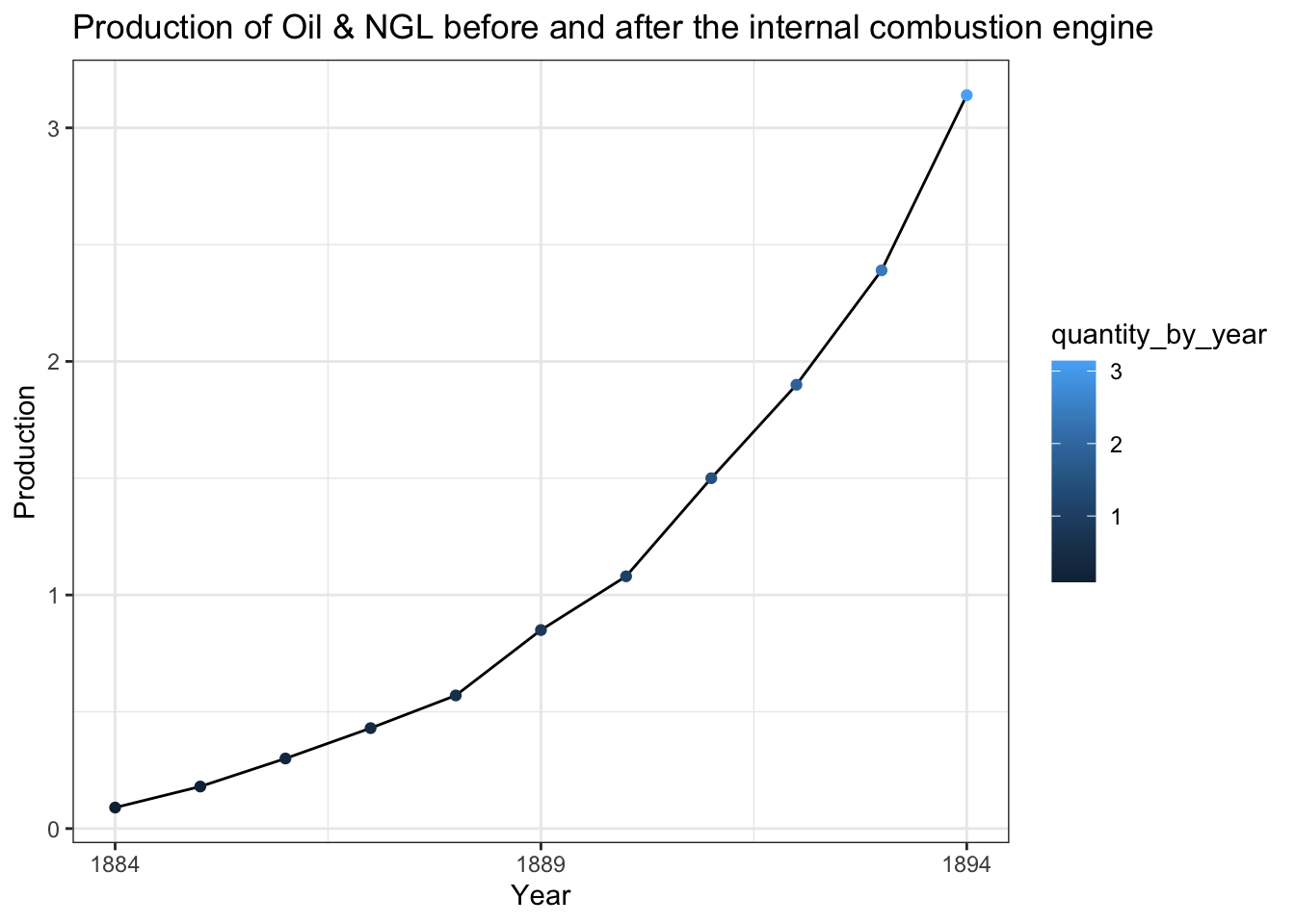
Q10: Two periods: (1)1854-1874, before the invention of internal combustion engine;(2) 1875-1894. Trends in the production of “Oil & NGL” and the emissions
df_cleaned|>filter(year>="1854"& year<="1894")|>group_by(year)|>summarise(emissions_by_year=sum(emissions))|>ggplot(aes(x = year, y = emissions_by_year)) +geom_line() +geom_point(aes(color = emissions_by_year)) +scale_x_continuous(breaks =seq(1854, 1894, 5)) +labs(title ="Emissons before and after the internal combustion engine",x ="Year",y ="Emissions(MtCO2e)") +theme_bw()
df_cleaned|>filter(year>="1854"& year<="1894")|>filter(commodity=="Oil & NGL")|>group_by(year)|>summarise(quantity_by_year=sum(quantity))|>ggplot(aes(x = year, y = quantity_by_year)) +geom_line() +geom_point(aes(color = quantity_by_year)) +scale_x_continuous(breaks =seq(1854, 1894, 5)) +labs(title ="Production of Oil & NGL before and after the internal combustion engine",x ="Year",y ="Production") +theme_bw()
Q11
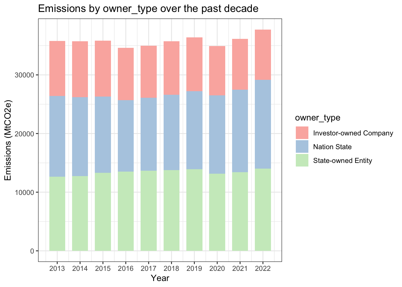
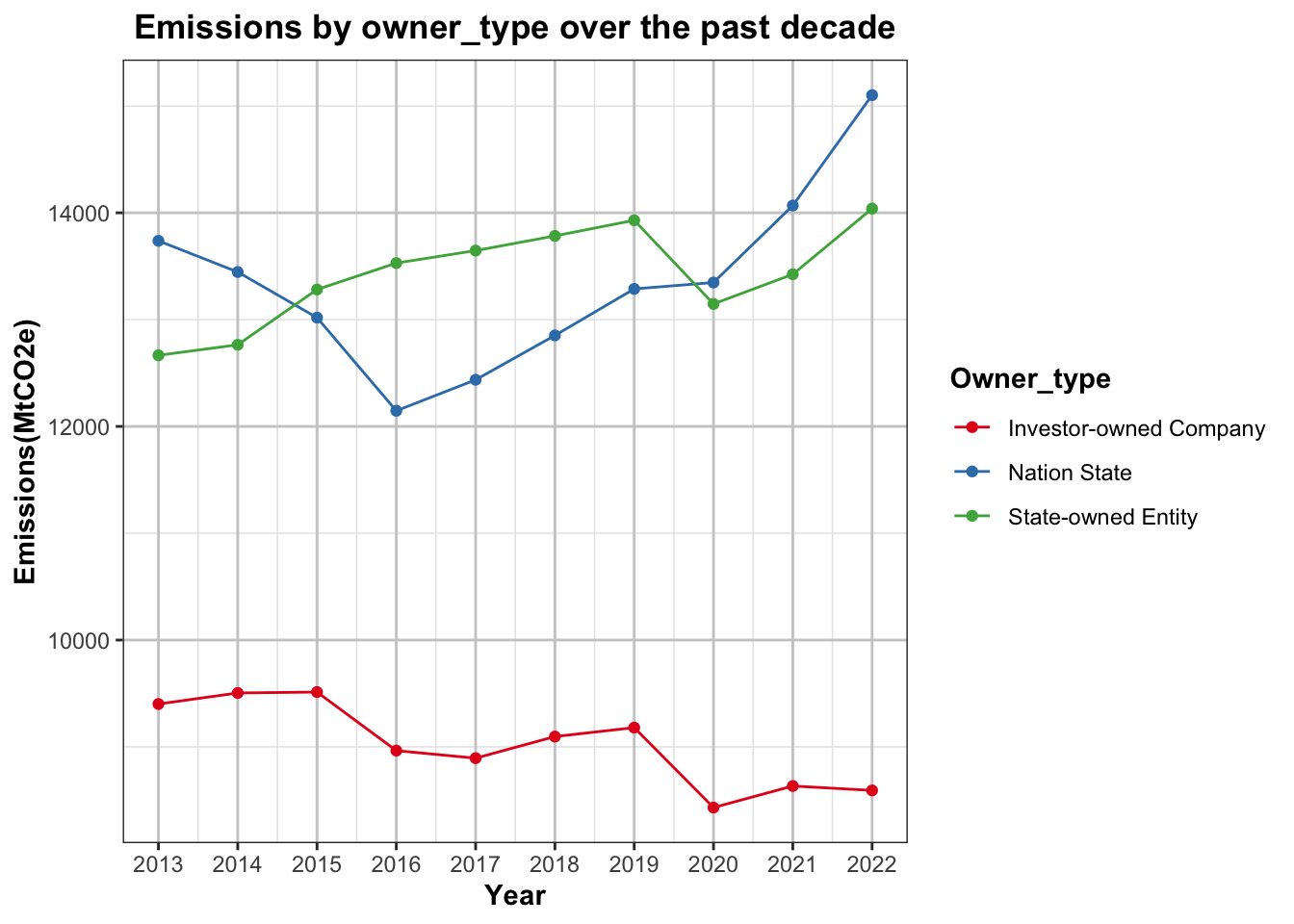
Q11: Trends in emissions by owner_type over the past decade.
df_cleaned |>filter(year >="2013") |>group_by(year, owner_type) |>summarise(total =sum(emissions)) |>ggplot(aes(x = year, y = total, fill = owner_type)) +geom_col(width =0.7) +scale_x_continuous(breaks =seq(2013, 2022, 1)) +scale_fill_brewer(palette ="Pastel1") +labs(title ="Emissions by owner_type over the past decade",x ="Year",y ="Emissions (MtCO2e)") +theme_bw()
`summarise()` has grouped output by 'year'. You can override using the
`.groups` argument.
df_cleaned|>filter(year>="2013" )|>group_by(year,owner_type)|>summarise(total=sum(emissions))|>ggplot(aes(x = year, y = total, color = owner_type)) +geom_line(aes(color = owner_type)) +geom_point(aes(color = owner_type)) +scale_x_continuous(breaks =seq(2013, 2022, 1)) +scale_color_brewer(palette ="Set1") +labs(title ="Emissions by owner_type over the past decade",x ="Year",y ="Emissions(MtCO2e)",color ="Owner_type") +theme_bw()+theme(plot.title =element_text(hjust =0.5, face ="bold"),legend.position ="right",legend.title =element_text(face ="bold"),axis.title =element_text(face ="bold"),panel.grid.minor =element_line(color ="grey90"),panel.grid.major =element_line(color ="grey80"))
`summarise()` has grouped output by 'year'. You can override using the
`.groups` argument.